Changing desktop background and display themes

Accomplishing that is trivial in any OS but it is a good idea to do it once in a while to break the monotony and keep things fresh.

Calculating Rg using VMD

I am working on a system with 60 copies of a molecule which has 1287 atoms in it. The script below loads the trajectory and calculates the radius of gyration of each copy.

mol new system.gro

for {set num 0} {$num < 201} {incr num} {
mol addfile cen_md_$num.xtc waitfor all
}

for {set i 1} {$i <61} {incr i} {
set start [expr 1 + 1287 * ($i-1) ]
set end [expr 1287 * $i]
puts "$start $end"
set sel [atomselect top "serial $start to $end"]
set filename [open "rg-dextran-number-$i.txt" w]
puts "Number of frames is [molinfo top get numframes]";
for {set frame 0} {$frame < [molinfo top get numframes]} {incr frame} {
animate goto $frame
$sel update
puts $filename [format "%8.3f" [measure rgyr $sel]]
}
close $filename
}

quit

Weighted Histogram Analysis Method - WHAM

WHAM is used extensively to calculate the free energy of a system along a properly chosen reaction coordinate in molecular dynamics simulations or monte carlo simulations. To be able to use WHAM you need to perform multiple simulations that cover the entire reaction coordinate to sample possible configurations. The choice of reaction coordinate constitutes a length discussion and is a topic of ongoing debate. So I encourage the reader to look it up elsewhere. After you have chosen a reaction coordinate and performed Umbrella Sampling or Free Energy Perturbation calculations, histograms corresponding to every window need to be extracted.

For the simple case of dragging a methane molecule from water into a lipid bilayer and out into water again, z axis is a good reaction coordinate if the lipid bilayer is on the x-y plane. With this set up, the z axis is split into discrete windows and the center of mass (COM) of the methane molecule is constrained (usually harmonic) to the center of every window. The length of windows and force constant of the constraint are chose such that the distribution of the z coordinate of the COM of methane overlaps with the distribution of the adjacent windows. This is a necessary prerequisite for using WHAM. Following the figure below, for a 60A long reaction coordinate a choice of 121 windows (each 0.5A and including both ends) will be plenty to ensure overlap of z coordinate distributions.

Collect z coordinate distributions and put them 121 files labeled window-001 to window-121.
Create a new file input.in that contains the following lines;

./window-001 -30.0 xx
./window-002 -29.5 xx
...
./window-120 +29.5 xx
./window-121 +30.0 xx

Here the first column is the file name, second is the mean value of that window and the third column needs to be filled with an integer but is irrelevant and not used by Alan Grossfield's implmentation of WHAM. Then run the following command

./wham 1 11 10 0.001 300 0 input.in freefile

where the inputs are

./wham hist.min hist.max num.bins tol Temp numpad infile outfile

Figure Source: http://www.utdallas.edu/~son051000/comp/FreeE.pdf

The output contains a plot for the potential of mean force (PMF). Pay particular attention to units since they depend on your input. WHAM's documentation can be found here [http://membrane.urmc.rochester.edu/sites/default/files/wham/doc.html].

Ubuntu grub rescue

Following are my notes while I successfully recovered Ubuntu 12.04-LTS from grub recovery mode.

I am using a Macbook Pro and trying to create a Ubuntu Live USB.

Create a Live USB using instructions from here.

http://www.ubuntu.com/download/desktop/create-a-usb-stick-on-mac-osx

This tells you how to work through grub rescue.

http://askubuntu.com/questions/197833/recovering-from-grub-rescue-crash

This video offers additional help

http://www.youtube.com/watch?v=8lod8sRb_6I

On a side note, if you ever accidentally delete /boot directory simply type the line below - just like this guy. Of course you need the find the appropriate linux-image-x.x.xx-xx-server and you do need to catch this blunder before rebooting.

sudo apt-get install --reinstall linux-image-2.6.32-42-server

Sorting by columns in R

Sorting columns in R is a breeze. If d is a matrix with 2 columns and you want to sort d by column 1, use the command order as below.

DNA simulation set-up with AMBER

I have been working on the structure and dynamics of single and double stranded DNA for some time now and below is a write up of an easy way to setup the simulations using the AMBER suite of software. Along with primary executables sander, pmemd, tleap and ptraj, AMBER comes with a number of other useful tools. One such tool is the nucleic acid builder (or nab). To create a 10mer poly-Adenosine poly-Thymidine, put the following text in a file called nuc.nab;

molecule m;
m = fd_helix( "abdna", "aaaaaaaaaa", "dna" );
putpdb( "nuc.pdb", m, "-wwpdb");

Then run these in the terminal

nab nuc.nab
./a.out

You should get a nuc.pdb file which contains the poly A-T double stranded DNA. Everything so far is available in more detail at http://ambermd.org/tutorials/basic/tutorial1/section2.htm

To get a single stranded poly-A DNA simply delete the lines corresponding to poly-T. To create stem-loop type configurations commonly found in RNA, do the following. Say you want the ssDNA

AAATAGAGCTAGTGAGGATTT

with the first 4 bp [AAAT] paired with the last 4 [TTTA or ATTT if you want to read from above]. For this I simply generate a double stranded DNA like so...

AAATAGAGCTAGTGAGGATTT
TTTATCTCGATCACTCCTAAA

Then delete the bases shown in red from the PDB file.

AAATAGAGCTAGTGAGGATTT
TTTATCTCGATCACTCCTAAA

Now you should have

AAATAGAGCTAGTGAGG
TTTA

This is the same as AAATAGAGCTAGTGAGGATTT but with the ends paired up. For the stem-loop conformation you should be able to use the parameter and topology files generated for the fully stretched single stranded DNA. You will have a long bond between  AAATAGAGCTAGTGAGG--and--ATTT. But this can be easily fixed with a quick minimization. 

Quick linear fitting with Gnuplot

From here ...

Toggle case of alphabets in /vi/ and console

tr 'a-z' 'A-Z' < contacts.txt

Case of letters in the file contacts.txt can be changed from lower to upper using the console command above. In vi the same can be achieved by switching to command mode and typing the tilde key on the letter of choice. For bulk edits visualization mode (Ctrl+v) works well. More information about this can be found at: http://vim.wikia.com/wiki/Switching_case_of_characters

Installing Octave on MacBook

Here are the notes I took while successfully installing Octave on MacBook 10.8.4

Exploring Apple Keynote

I am trying out Apple's Keynote to see what the fuss is all about. dashkards.com/keynote is a great site where I found this:

C style formatting in R

Numbering/naming files in a controllable format is important when making animations of a series of plots (by using animate for example). When the plots are being generated in R, there is an easy way to control the names of the output files as shown below;

The advantage here is that when you feed in files with the same base.name and numbered 000..100 (instead of 0..100), the command convert automatically reads them in increasing order w/o you relying on time stamps and such. 

Linux terminal colors (Console, ls and vi)

The lines below when put in my .bashrc file greatly improved the readability - I essentially turn the color scheme off.

# Below is from http://mylinuxbook.com/ubuntu-command-line-prompt-colour/
if [ "$color_prompt" = yes ]; then
    PS1='${debian_chroot:+($debian_chroot)}\[\033[0;31m\]\u@\h\[\033[00m\]:\[\033[01;34m\]\w\[\033[00m\]\$ '
else
    PS1='${debian_chroot:+($debian_chroot)}\u@\h:\w\$ '
fi

alias ls='ls --color=none'

Further these lines in .vimrc file were of great help.

syntax on
colorscheme desert

ImageMagick's display

On Linux terminal the command /display/ simply displays a figure w/o any resizing. This can get cumbersome when dealing with large images. However, a simple resize option simplifies life:

display -resize 1080x\> figure.png

where the width is being resized to 1080 pixels while the height is automatically assigned. This link suggests using this approach only for downsizing images. 

Interesting thoughts...

Input arguments for /scanf/ type commands

For executables that require user-input, data can be fed in the following manner:

echo 5|pdb2gmx -f box.his.pdb -o box150

where 5 is the input argument that would otherwise have to be given after pdb2gmx takes its time running through its code that comes before a scanf type statement. This approach saves time and automates the process provided you know which argument to feed in. You can extend this any number of arguments like so...here 5 is argument 1 and 50 is argument 2.

echo 5 50|pdb2gmx -f box.his.pdb -o box150

Link between common distributions

People dealing with large data sets often find themselves using one of the many standard distribution functions to explain their data. Some of the more commonly used distributions are binomial, Gaussian and Poisson. Interestingly the latter two can be derived from the binomial distribution in that the Poisson distribution is a limit of the binomial distribution and the Gaussian is a limit of the Poisson. The derivations below (conveniently lifted from the web) elaborate.

Source:

http://www.roe.ac.uk/japwww/teaching/astrostats/astrostats2012_part2.pdf

http://www.physik.uzh.ch/~psaha/pda/

Installing Citrix on a 64bit Linux box (Ubuntu)

I had previously managed to install Citrix on a 32bit Linux box with little pain but I had a very different experience when dealing with 64bit Linux. Anyway I solved the issues and got it running. Below are the steps involved. You need Citrix if you see a screen similar to the ones below.

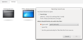
- Download 64bit Citrix. Supplied either by your institution or a relevant one at http://www.citrix.com/downloads/citrix-receiver/linux/receiver-for-linux-121.html
- Run dpkg -i ...deb. It will fail. Let it fail.
- Edit /var/lib/dpkg/info/icaclient.postinst so that this line shows up
 if [ "$arch" = "x86_64" -a "$op_system" = "Linux" ]
- Run dpkg --configure icaclient [no more arguments needed]
- sudo ln -s /etc/ssl/certs/Thawte_Premium_Server_CA.pem /location/of/ICAClient/keystore/cacerts/

That's it!

Make sure dependencies are all of same arch (x86).
nsplugin wrapper is an example for that. This depends on libc6.i386 and other libs.
Install libc6. This will iron out other problems. I thank Zach and Mike for their patience while working this out.

VMD 'measure hbonds' syntax

The figure below makes it easy to remember the syntax of VMD's measure hbonds command.

Subsetting data with string matching in R

Getting a subset from a larger pool of data is a major strength in R. This subsetting can be based on numbers or strings; the latter being more challenging. String matching (using grep, grepl, sub) and subsetting (using, well, subset in R) are two separate feature and one can combine them to great effect. Details of what grep, grepl etc can do are at
http://stat.ethz.ch/R-manual/R-devel/library/base/html/grep.html . This site
http://atomicules.co.uk/2010/10/09/invert-a-subset-selection-when-using-grepl-in-r.html
was of great help when I wanted (had) to use grepl in subset but I also wanted to use the invert feature available only in grep and not in grepl. Turns out grepl returns a vectors of T and F which can be easily inverted with a simple !grepl(...)

Area under a curve

R has a neat way to calculate area under a curve (whether a function/equation or a trend line). The example below describes the two ways in which this can be achieved. rollmean requires library(zoo).

Making and filling grids with R

I had a table with 64 rows and 130 columns and I needed to map a third dimension as a simple X on the 2D plot based on some criteria. I got this done in R using a code similar to the one below.

Contact Maps using VMD

Contact maps are a quick way to identify residues of a protein (or monomer) that interact with residue from another protein, ligand or monomer. The script below helps obtain a distance list:

set seg1 [atomselect top "segname SG03 and name CA"]

set seg2 [atomselect top "segname SG04 and name CA"]

set file [open "Contact_map.dat" w]

set list1 [$seg1 get index]

set list2 [$seg2 get index]

foreach atom1 $list1 {

        foreach atom2 $list2 {

                set index1 [atomselect top "index $atom1"]

                set index2 [atomselect top "index $atom2"]

                set resid1 [[atomselect top "index $atom1"] get resid]

                set resid2 [[atomselect top "index $atom2"] get resid]

                set resnm1 [[atomselect top "index $atom1"] get resname]

                set resnm2 [[atomselect top "index $atom2"] get resname]

     puts $file "$resnm1 $resid1 $resnm2 $resid2 [veclength [vecsub [measure center $index1] [measure center $index2]]]"

                $index1 delete

                $index2 delete

        }

puts $file " "   # I include this line to make it easier to make contour plots using gnuplot.

}

close $file

Aligning hexameric proteins along an axis

This tcl script aligns a hexamer such that its central axis is aligned along the y-axis.


set all [atomselect top protein]
$all moveby [vecscale [measure center $all] -1]

set res10 [atomselect top "resid 10"]
set res40 [atomselect top "resid 40"]

set cenres10 [measure center $res10]
set cenres40 [measure center $res40]

set vector [vecsub $cenres10 $cenres40]

$all move [transvecinv $vector]
$all move [transaxis z 90]

foreach i {A B C D E F} {
        set chain [atomselect top "chain $i and protein and resid 4 to 105"]
        $chain writepdb chain$i.pdb
}

This script is also applicable to trimers, tetramers and other aggregates that have a well defined central axis.

Curve fitting in R

This is a simple example of a linear fit where a perfect fit is distorted with the help of a gaussian function. This data is then fit to a linear model. The most important factor determining the success of a fit is the model equation and the second most important factor is suitable starting values of the fit variables (a and b in this case). Further, if you assign the output to a variable called fit, values a and b can be extracted using:

fit < - nls
coef(fit)[1]
coef(fit)[2]

Saving data frames in R

If 'df' is your data frame,
save(df,file="yourfile.rdf",ascii=TRUE)
save the data frame in to a .rdf file which is readable. Although the file as lot more data than you might want, loading the file back into R irons out any wrinkles.
load("yourfile.rdf")
http://stackoverflow.com/questions/8345759/how-to-save-a-data-frame-in-r

Edit Jan 2014
If however you really want to avoid additional lines in the saved file, try the following:
write.table(df,filename,row.names=FALSE,col.names=FALSE)
This should produce a clean file with your data in a neat column.

Speaker and Mic settings on Ubuntu Linux

Although Skype and Google video get installed fairly easily on Ubuntu, bad sound settings could be a show stopper. Alsamixer controls the sound and mic and can be force rebooted using:

alsa force-reload
or
alsa reload

This usually fixes most problems. Other useful links:
http://askubuntu.com/questions/164518/hard-resetting-alsa-configuration
http://chriscarey.com/wordpress/2008/07/01/reset-alsa-sound-on-linux/
http://ubuntuforums.org/showthread.php?t=1068612
http://forums.bodhilinux.com/index.php?/topic/3800-solved-how-does-a-user-restart-alsa-without-rebooting/

Mapping 3d data on a 2d color map

Gnuplot has a very easy and straightforward way to convert a x-y-z data into a 3d plot or a 2d color map. Let's write the data in the form;
1 1     0.0
1 2     0.4451
1 3     0.4249

2 1     0.13142
2 2     0.0
2 3     0.983

3 1     xxx
3 2     xxx
3 3

A space between chunks of data is important. Using commands below you can get a 2d plot;

set size square
set pm3d map    # Remove the word 'map' to get a 3d plot
set xrange [1:261]  # Change the range to suit your needs
set yrange [1:261] 
splot 'all.dat'

Reducing the file size of PDF documents

gs -sDEVICE=pdfwrite -dCompatibilityLevel=1.4 -dPDFSETTINGS=/screen -dNOPAUSE -dQUIET -dBATCH -sOutputFile=output.pdf input.pdf

I recently made a nice pdf figure using R but the file was 18Mb heavy. With 7 such figures my manuscript was easily crossing the 100Mb mark which felt rather unnecessary. The command above scales down the18Mb file to a tenth of its size. Since these figures are based on vectors, scaling down the file size has little to no impact on the quality of the figure when zoomed in. gs is turning out to be far more potent than I initially thought.

Sweave, R and Latex

If you use R for your statistical analysis and graph plotting needs and then use those figures in your Latex documents, you will find this interesting. Sweave is a package in R which lets takes in an .rnw file (which contains usual text from a tex document with R commands embedded in it), compiles it (in R) and gives out a tex file. This tex file can in turn be compiled by pdflatex (if you have figures) or plain latex to get a properly formatted pdf/ps/dvi file with relevant R output. There are many excellent examples on the interwebs and I strongly recommend using Sweave right away.  The beauty of this approach is that on can save a lot of time by not spending on choosing the appropriate dimensions of a a png or an eps output. Sweave does it for you.

Edit: If you want to insert a R-generated figure then add this to your tex file:

\begin{figure}
\begin{center}
<>=
out3 <- br="" i="" lm="" x="" y="">plot(x, y)
@
\end{center}
\end{figure}


If you want to insert text from R but properly tabbed and with all the ampersands added, then add these lines to your tex file:

<>=
library(xtable)
print(xtable(foo, caption = "ANOVA Table", label = "tab:one",
         digits = c(0, 0, 2, 0, 2, 3, 3)), table.placement = "tbp",
         caption.placement = "top")
@

Manipulating dihedral angles in VMD

VMD's scripting interface is quite powerful. It has a trans bond command which gives the transformation matrix required to achieve desired dihedral rotation. If you want to edit the dihedral 1-2-3-4 (i.e. rotate around bond 2-3), then you first select the set of atoms on which the transformation is to be applied; 1,2,5,6,7,8,9 in this case. To this selection you apply the transformation;

$moveselection move [trans bond [lindex [$a1 get {x y z}] 0] [lindex [$a2 get {x y z}] 0] 10 deg]

trans bond expects only the atom indices. The value 10 indicates the magnitude and sign of change to the dihedral 1-2-3-4. deg says the change should be in degrees and not radians. To get a nice picture of rotation around a bond use this script:

set movesel [atomselect top "index 1 2 5 6 7 8 9"]
for {set i 0} {$i <360 } {incr i 10}
{
$movesel move [trans bond [lindex [$a1 get {x y z}] 0] [lindex [$a2 get {x y z}] 0] 10 deg]
render TachyonInternal [format "rotate%03d.tga" $i]
}

Joining multiple pdf files in Linux

gs -dBATCH -dNOPAUSE -q -sDEVICE=pdfwrite -sOutputFile=finished.pdf file[1-3].pdf

This is a great way to join many pdf files into one file. Mac's Preview has another way to do the same but in a much easier drag-and-drop fashion. The line below in my .bashrc file helps automate the concatenation process.

alias join='gs -dBATCH -dNOPAUSE -q -sDEVICE=pdfwrite -sOutputFile=awkwardName.pdf'

time and script

These are great commands in Linux while debugging and timing codes.

Combining figures into one PDF file

convert -compress JPEG *.jpg output.pdf
convert -compress Zip *.jpg output.pdf

Both the commands join a bunch of jpeg files into one pdf file. This came in handy recently. Dropping the compress flag and its options gave a smaller file. Might look into it later.

convert *.jpg output.pdf

Bibtex being bibtex

Do you notice any difference between this:


@article{Dashnau2007Computational,
    abstract = {.....}
    author = {Dashnau, J. L. and Vanderkooi, J. M.},
    journal = {J. Food Sci.},
    month = jan,
    number = {1},
    pages = {R001--R010},
    title = {{Computational Approaches to Investigate How Biological Macromolecules Can Be Protected in Extreme Conditions}},
    volume = {72},
    year = {2007}
}

and this:


@article{Dashnau2007Computational,
    abstract = {.....}
    author = {Dashnau, J. L. and Vanderkooi, J. M.},
    journal = {J. Food Sci.}
    month = jan,
    number = {1},
    pages = {R001--R010},
    title = {{Computational Approaches to Investigate How Biological Macromolecules Can Be Protected in Extreme Conditions}},
    volume = {72},
    year = {2007}
}

Well, I couldn't either. Notice the comma at the end of the journal entry? Well without the comma Bibtex ignores the ensuing metadata creating problems when compiling your document. Something to be careful about.

Batch cropping images using Mogrify

The command 'mogrify' can crop multiple images simultaneously. Sample case is below.
mogrify -crop WidthxHeight+x+y        images*.png
mogrify -crop 2796x983+429+327        images*.png
The values of width, height, x and y can be obtained by opening an image in Gimp and selecting the rectangle of interest.

Firefox/Thunderbird already running but not responding

Firefox and Thunderbird can sometimes give this error when you restart a linux box or when you try to make multiple log ins into a shared file system. The result is that Firefox/Thunderbird will not open. The causes for this are not entirely clear to me but I found a solution. Simply delete the .parentlock file in both cases and restart the service. Locations for this file are as follows:
Firefox: ~/.mozilla/firefox/xxxxx.default/.parentlock
Thunderbird: ~/.thunderbird/xxxxx.default/.parentlock
Since both the folders and files start with a dot, they are not visible with a simple
ls -lrt
You have to use
ls -lrta

Emacs Primer

I decided just a little while ago that it was time I learned how to use a text editor other than vi. Below are my notes as I keep learning more about Emacs.

Open a new file: emacs newfile.txt &

Starting writing in the file.

Save: ctrl x s
Search Forward: ctrl s
Search Reverse: ctrl r

Exit emacs: ctrl x c

Select Region:      ctrl space and arrows
Mark Activate:      ctrl space
Mark Deactivate: ctrl space or ctrl g
Select All: ctrl x (wait) h

Delete Region: ctrl w
Copy Region:   Esc  w
Paste buffer: ctrl y

Delete till end of sentence: ctrl k

Delete line: ctrl S backspace

Delete next word: Esc d

Undo last action: ctrl _ (underscore)

Jump to end of file: Esc >
Jump to start of file: Esc <
Go to line 10: Esc x 10   

List all buffers: ctrl x (leave ctrl) b

Split screen:                                   ctrl x (leave ctrl) 2
Close all but current buffer:     ctrl x (leave ctrl) 1
Close only the current buffer:  ctrl x (leave ctrl) 0

Repeat 9 times: ctrl u (leave ctrl) 9
Type - 9 times: ctrl u (leave ctrl) 9 -

If you start a command and then decide you don't want to complete it, type C-g to cancel it.

http://doors.stanford.edu/~sr/computing/emacs.html
http://www.nbcs.rutgers.edu/newdocs/unx01101/unx01101.php3
http://dept.cs.williams.edu/~kim/cs136/s04/emacs.html

Edit: Dec 28, 2012
I was writing a manuscript in Emacs and the bibtex reference key had a beta symbol which meant that I had to type this into Emacs;   Kheterpal2000Aβ and not Kheterpal2000$\beta$. To do this I copied the following two lines into ~/.emacs and solved my problem. Thanks to this site.

(global-set-key (kbd " a") "α") ; F9 followed by a
(global-set-key (kbd " b") "β")

Java script to get Long/Lat in Google Maps

javascript:alert(window.gApplication.getMap().getCenter());

Latex Template

Reminding myself of every detail in the assigning of packages and page type in Latex seems like a bit of a chore. So I copied the following from a working .tex file to reduce redundancy.

\documentclass[12pt,doublespace]{article}

\usepackage[top=3cm,bottom=3cm,left=2.5cm,right=2.5cm]{geometry}

\usepackage{rotating}

\usepackage{apacite}

\begin{document}

\title{}

\author{

Name

\small Affiliation

\and

New Name

\small Affiliation

}

\maketitle

\begin{abstract}

...

\end{abstract}

\section{}

Main body

\end{document}

pdflatex vs pdftex

I have a document with lot of .eps figures embedded in it. These figures were of high quality but also large size. To cut down on the size I converted them to .png which were a tenth of the .eps format. Now using
latex file.tex (with eps figures)
worked well. But to use .png figures I thought I had to use pdftex.
pdftex file.tex (with png figures)
Turns out I should have used pdflatex instead. I ended up losing quite some time on this. The switch to pdflatex did the job and gave me a file which was a tenth of the original size. More on this from here:

"pdftex expects the file to be plain TeX. pdflatex expects it to be LaTeX. These
are two different dialects of TeX. You do not expect a C compiler to work with
Java, do you?

Note that in practice pdftex and pdflatex are often the same command, which
analyzes how it was called to switch to the proper input language. On some
systems gcc behaves in the same way, compiling C if it is called as gcc or
Fortran if it is called as gfortran."

Bottom line, figures can be heavily compressed by converting them to png format w/o a large loss in clarity; and pdflatex can handle png figures. Even if there is a loss of clarity, this is usually just fine for supporting information; maybe not so much for main article.

Enough said...

Handling references using BibTex

Scientific journals with arbitrary requirements for reference styles can be a source of great heart-ache. When writing articles using Latex-BibTex, ability to handle reference styles can be useful. These articles are a great starting point to learn more about this:

http://amath.colorado.edu/documentation/LaTeX/reference/faq/bibstyles.html#styles

http://chenfuture.wordpress.com/2007/09/24/diy-your-bibtex-style-file/

http://www.math.washington.edu/tex-archive/macros/latex/contrib/custom-bib/merlin.pdf

Controlling axis properties in R

http://www.programmingr.com/content/controlling-margins-and-axes-oma-and-mgp/

The mgp option
In addition to changing the margin size of your charts, you may also want to change the way axes and labels are spatially arranged. One method of doing so is the mgp parameter option. The mgp setting is defined by a three item vector wherein the first value represents the distance of the axis labels or titles from the axes, the second value is the distance of the tick mark labels from the axes, and the third is the distance of the tick mark symbols from the axes. As with the oma option discussed above, the distances are given in line widths. The defaults for the mgp setting are c(3, 1, 0). The examples below illustrate the effects of changing the various mgp values. Note: the mgp.axis() function in the Hmisc package can be used to change these settings for each axis individually.

ImageJ Resources

http://rsbweb.nih.gov/ij/
http://www.fmhs.auckland.ac.nz/sms/biru/facilities/analysis_resources.aspx

Learning ImageJ

ImageJ is a fantastic light-weight tool to analyze and manipulate images. I needed to use it for quickly analyzing microscopy images. Here I will list features of ImageJ that I found particularly useful for my purposes:
- I took a bunch of images at various gains to find out the point where bleaching starts occurring. So I have a series of images in which the pixel intensity varies from 0 to 255.

ImageJ allows me to load the images as a stack and calculate the maximum pixel value in each image by selecting the whole image and hitting 'm' (for measure). Plotting the maximum value gives this:

So, bleaching occurs somewhere between a gain of 450 and 475.

Print page-range using lpr

I use the extremely light-weight pdf viewer, xpdf. For some unknown reason, I cannot print pages from xpdf. A nice workaround I found was with dear old lpr which can print a range of pages thus;
lpr -P HP_LaserJet_6MP file.pdf -o page-ranges=2-5
lpstat -a # Gives the status (and names) of all the connected printers

Batch processing images in Gimp

Over the past few weeks I've had to apply a specific set of changes to a large number of images. Doing this repeatedly took a great toll on my soul and Gimp came to my soul's rescue. Take a read at this and this and help yourself.

Memory convservation in R

Depending on how large a data set you are handling, R can take up large swaths of your RAM and slow down other processes. It is therefore a good idea to remove unused variables.
ls()  # Gives the list of variables/arrays currently in use.
rm(list=ls()) # Removes all the variables and frees up memory.
Useful links:
 http://www.matthewckeller.com/html/memory.html

Benchmarking Simulations

It is always a good idea to benchmark your simulations and select the optimal number of cores for your simulations. This exercise greatly reduces wastage of resources and time. The script below helps with the setup. You need files conf.in and template.pbs

for i in 24 48 96 192 240 576 960 1200; do
        mkdir scaling$i
        cp conf.in scaling$i
        sed 's/xxx/'$i'/g' template.pbs > scaling${i}/sub.pbs
        echo "cd scaling$i";
        echo "aprun -n $i $namd conf.in 2>&1 1> conf.out &";  
        echo "cd \$PBS_O_WORKDIR";
done

exit;



----- Template.pbs ------
#PBS -q debug
#PBS -l mppwidth=xxx
#PBS -l walltime=00:30:00
#PBS -N scaling
#PBS -S /bin/bash
#PBS -j oe

namd=/usr/common/usg/namd/2.8/bin/namd2
cd $PBS_O_WORKDIR
aprun -n xxx $namd conf.in 2>&1 1> conf.out

Making 2D heat-maps of protein secondary structure

I needed to make 2D heat-maps of protein structure with time on x-axis and protein residues on y-axis. This helps to see the time evolution of structure quite nicely. This is easily accomplished by loading the trajectory in VMD and sourcing the file ss_traj.tcl and going through your entire trajectory once. This creates a buffer with all the structure information. ss_traj.tcl creates a ss_traj.dat file which has the structure information. This ss_traj.dat file is then used by ss_plot.c, after compilation of course, to generate a .ps file with the desired output. All this is explained quite well here. I made a personal copy of the files here:
ss_traj.tcl
ss_plot.c
Sample ss_traj.dat file.

Once you have the output in .ps format you can do interesting things to change the file. The 7th line has the scaling information. The width and height of the output were not to my satisfaction; so I changed the scaling factors to adjust the display. Also the executable could crash when running due to memory requirements. Simply change the dimensions of the array in ss_plot.c according to your needs.

Reading/processing multiple files in R

j<-1;
for (i in seq(300,390,15)) {
df<-read.table(paste("sasa",i,".txt",sep=``));
# Files are named "sasa300.txt" for ex.
tab[j,]<-cbind(i,mean(df[,2]),sd(df[,2]));
print(tab[j,]);
j<-j+1;
}
> tab
     [,1]     [,2]      [,3]
[1,]  300 3408.514  96.48097
[2,]  315 3422.388 119.14861
[3,]  330 3391.590  81.57252
[4,]  345 3424.176  84.84211
[5,]  360 3394.205 100.37193
[6,]  375 3462.469 122.60486
[7,]  390 3438.328  92.70519

Quick and dirty way to plot error bars in R

If you have data that looks as follows, a one line command can draw error bars to the plot.
-x---T-----y-------------error-----
p5 315 2.513402 0.5711628                                                      
p5 330 2.173868 0.4711594                                                      
p5 345 2.132954 0.634045                                                       
p5 360 2.092686 0.4851832                                                      
p5 375 2.966971 0.9165328                                                      
p5 390 2.214886 0.4288291

r<-read.table("data.txt")
plot(r[,2],r[,3],ylim=c(0,4))
lines(r[,2],r[,3])
for(i in 1:length(r[,1])) {segments(r[i,2],r[i,3]+r[i,4],r[i,2],r[i,3]-r[i,4])}

I am drawing a simple line from (x,y+err) to (x,y-err). The result is not as fancy as other efforts but it is enough for my purposes.

Using psfgen to delete unwanted atoms in simulations

psfgen's user manual can be found here.

Adding labels to figures using ImageMagick

This is a 1200x1200 pixel blank file to which I added labels as an exercise in using the annotate flag in ImageMagick's convert.
 
convert blank.gif -pointsize 50 \
-gravity south -append -annotate +000+000 '0s' \
-gravity south -append -annotate +100+100 '1s' \
...
-gravity south -append -annotate +900+900 '9s' \
-gravity north -append -annotate +000+000 '0n' \
-gravity north -append -annotate +100+100 '1n' \
...
-gravity north -append -annotate +900+900 '9n' \
-gravity northwest -append -annotate +000+000 '0nw' \
-gravity northwest -append -annotate +100+100 '1nw' \
...
-gravity northwest -append -annotate +900+900 '9nw' \
-gravity northeast -append -annotate +000+000 '0ne' \
-gravity northeast -append -annotate +100+100 '1ne' \
...
-gravity northeast -append -annotate +900+900 '9ne' \
out.png

Joining images using Latex

Do not forget to use pdflatex (not pdftex) to compile tex files which contain non-eps figures.
 
\documentclass{article}
\usepackage{rotating}
\usepackage{graphicx,subfig}

% Default margins are too wide all the way around. I reset them here
\setlength{\topmargin}{-.5in}
\setlength{\textheight}{9in}
\setlength{\oddsidemargin}{.125in}
\setlength{\textwidth}{6.25in}

\begin{document}


\begin{sidewaysfigure}
\begin{tabular}{cc...c}
\includegraphics[scale=0.10, bb= 0 0 669 834]{view1_mol0} &
\includegraphics[scale=0.10, bb= 0 0 669 834]{view1_mol10} \\

\includegraphics[scale=0.10, bb= 0 0 669 834]{view0_mol0} &
\includegraphics[scale=0.10, bb= 0 0 669 834]{view0_mol10} \\

\includegraphics[scale=0.10, bb= 0 0 669 834]{view2_mol0} &
\includegraphics[scale=0.10, bb= 0 0 669 834]{view2_mol10} \\

\end{tabular}
\end{sidewaysfigure}

\end{document}

Joining images using ImageMagick's convert

convert +append list_of_figures out_1.png
convert +append list_of_figures out_2.png
convert +append list_of_figures out_3.png
convert -append out_1.png out_2.png out_3.png final_out.png

+append puts images side by side while -append adds them top down.
convert -border 2x2 in.png out.png
This puts a light border around images which comes in handy when creating a grid of images from a bunch of individual images which have no border.

Empty plots in R

When plotting a grid of graphs in R, I needed leave some cells empty. For this the following commands come handy;

plot(0,xaxt='n',yaxt='n',bty='n',pch='',ylab='',xlab='')

plot.new()

grid.newpage()

grid()

Subsetting in R

Following are some example of subsetting in R I have used recently.


> head(crystal)
    V1     V2      V3      V4
1 1ACJ PHE120 290.980 289.101
2 1ACJ PHE153 307.673 283.814
3 1ACJ PHE155 296.153  89.152
4 1ACJ PHE186 311.606 292.186
5 1ACJ PHE187 298.920 270.613
6 1ACJ PHE197  66.678 323.351

>subset(crystal, crystal$V2=="PHE330" & grepl("^2A",crystal$V1))

http://www.ats.ucla.edu/stat/r/faq/subset_R.htm
http://stackoverflow.com/questions/2125231/subsetting-in-r-using-or-condition-with-strings

Charmm2lammps

Charmm2lammps.pl is a useful little code which takes in forcefield [top/par], psf and pdb files in Charmm format and converts them to Lammps data and sample input file. This is extremely useful for running simulations in the much better written MD code, LAMMPS. While trying to simulate a polymer chain I came across a very interesting feature in charmm2lammps; it really expects the force constant in the forcefield parameter file to be non-zero. This works just fine when you never want to specify angle/dihedral parameters to free chains. But when you want to control the parameters in between runs, it is a good idea to define all the angle and dihedrals and then decide to turn them off/on in LAMMPS by setting the force constant to 0/nonzero.

Compiling C programs on Ubuntu

On Ubuntu, it turns out, this does not work
gcc -lm code.c
but this does
gcc code.c -lm

Running job on clusters continuously

Here is a way to run jobs on cluster in a continuous fashion. This example addresses NAMD jobs but should also work for others.

Labeling figures

http://www.imagemagick.org/Usage/annotating/
This website offers a  nice way to add labels to images that "convert" can handle. I thought it was a nice idea to have my name on figures I generate.

Public folder on Dropbox

http://dl.dropbox.com/u/65895350/

Extracting coordinates of protein from a simulation

set dir [pwd]
mol new     ${dir}/ache.psf       type {psf}
mol addfile ${dir}/ache.pdb       type {pdb} waitfor all
mol addfile ${dir}/acheminnpt.dcd type {dcd} waitfor all

set molnum 0
set skip 1
set backframe0 [atomselect $molnum backbone frame 0]

for {set i 0} {$i < [molinfo $molnum get numframes]} {incr i $skip} {
set pro  [atomselect $molnum protein  frame $i]

# Change 'protein' to "resid N to Z" to suit your needs.
set back [atomselect $molnum backbone frame $i]
set trans_mat [measure fit $back $backframe0]
$pro move $trans_mat
set k [expr $i/$skip]
$pro writedcd ${dir}/dcd/project-pdb-$k.dcd
}

Now generate a protein-only psf file. At this stage you should have n number of dcd files. To join them all in to one dcd file,

mol new    ${dir}/ache_protein.psf
set pro_frames [expr [molinfo $molnum get numframes]/$skip ]
for {set j 0} {$j < $pro_frames} {incr j 1} {
mol addfile ${dir}/dcd/project-pdb-$j.dcd
}
set top [molinfo top]
animate write dcd {${dir}/dcd/project_protein.dcd} beg 0 end [expr $pro_frames - 1] skip 1 [molinfo top]

The last step is where the individual files are stitched together.

Installing Gimp on Ubuntu 11.1

Last month I installed Gimp on Ubuntu 11.1 which dropped Gimp since they deemed it too complex for new linux converts. Since this was last month I don't remember all the steps I took but I did copy the commands to a file and they might come handy in future. Here they are...

   69  sudo add-apt-repository ppa:matthaeus123/mrw-gimp-svn
   71  sudo apt-get install gimp gimp-data gimp-plugin-registry gimp-data-extras
   73  sudo add-apt-repository ppa:lucid-bleed/ppa
   74  sudo add-apt-repository ppa:matthaeus123/mrw-gimp-svn
   79  mkdir gimp
   80  cd gimp/
   81  wget ftp://ftp.gimp.org/pub/gimp/v2.7/gimp-2.7.2.tar.bz2
   82  tar xjf gimp-2.7.2.tar.bz2
   83  export PATH=/opt/gimp-2.7/bin:$PATH
   84  export PKG_CONFIG_PATH=/opt/gimp-2.7/lib/pkgconfig
   85  export LD_LIBRARY_PATH=/opt/gimp-2.7/lib
   86  cd gimp-2.7.2/
   87  ./configure —prefix=/opt/gimp-2.7
   89  ./configure
   90  cd ..
   92  sudo apt-get install git
   93  git clone git://git.gnome.org/babl
   94  cd gimp-2.7.2/
   95  ./configure --prefix=/opt/gimp-2.7
   96  cd ..
   97  ./autogen.sh --prefix=/opt/gimp-2.7
   99  cd babl/
  100  ./autogen.sh --prefix=/opt/gimp-2.7
  101  make -j5
  102  cd ../gimp-2.7.2/
  103  ./configure --prefix=/opt/gimp-2.7
  104  cd ../babl/
  105  cd ..
  106  git clone git://git.gnome.org/babl
  107  ./autogen.sh --prefix=/opt/gimp-2.7
  108  sudo apt-get install libtool
  109  ./autogen.sh --prefix=/opt/gimp-2.7
  110  cd babl/
  111  ./autogen.sh --prefix=/opt/gimp-2.7
  112  make -j5
  113  sudo make install
  114  cd ../gimp-2.7.2/
  115  ./configure --prefix=/opt/gimp-2.7
  116  cd ..
  117  wget ftp://ftp.gimp.org/pub/gegl/0.1/gegl-0.1.6.tar.bz2
  118  tar -xjf gegl-0.1.6.tar.bz2
  119  sudo apt-get install libjpeg62-dev libopenexr-dev librsvg2-dev
  120  cd gegl-0.1.6/
  121  ./configure --prefix=/opt/gimp-2.7
  122  sudo make install
  123  cd ..
  124  ls
  125  cd gimp-2.7.2/
  126  ./configure --prefix=/opt/gimp-2.7
  127  sudo apt-get install libtiff4-dev python-dev python-gtk2-dev
  128  ./configure --prefix=/opt/gimp-2.7
  129  which gimp
  130  sudo apt-get install libexif-dev liblcms1-dev
  131  ./configure --prefix=/opt/gimp-2.7
  132  make -j5
  133  make install -j5
  134  sudo make install -j5
  135  ls /opt/gimp-2.7/bin/gimp-2.7
  136  /opt/gimp-2.7/bin/gimp-2.7
  137  history > ~/gimpinstallcommands.dat

Making movies with VMD/PyMol

These two scripts help greatly in making and handling movies. I need scripts instead of the GUI because most of my data is on machines on the other coast and it gets rather cumbersome to pull a gigantic trajectory file just to see a quick snapshot of the system. I could make PDB (or better dcd) files of parts of trajectory I am interested in, but I will need to make movies at some point.

view_change_render.tcl
trajectory_movie.tcl
http://www.myofilament.org/documents/howto/modeling/VMD_Tcl.htm

PyMol uses get_view and "set view" commands to save and retrieve views of molecules. VMD handles things a little differently. It needs 4 parameters per view. They are [rotate/center/scale/global]_matrix. Saving and retrieving are done by processes below. They have been taken from view_change_render.tcl
I added the last part get_vp to see what the view point actually looks like (similar to get_view in PyMol).

proc save_vp {view_num} {
  global viewpoints
  if [info exists viewpoints($view_num)] {unset viewpoints($view_num)}
  # get the current matricies
  foreach mol [molinfo list] {
    set viewpoints($view_num,$mol,0) [molinfo $mol get rotate_matrix]
    set viewpoints($view_num,$mol,1) [molinfo $mol get center_matrix]
    set viewpoints($view_num,$mol,2) [molinfo $mol get scale_matrix]
    set viewpoints($view_num,$mol,3) [molinfo $mol get global_matrix]
  }
} 

 proc retrieve_vp {view_num} {
  global viewpoints
  foreach mol [molinfo list] {
    if [info exists viewpoints($view_num,$mol,0)] {
      molinfo $mol set rotate_matrix   $viewpoints($view_num,$mol,0)
      molinfo $mol set center_matrix   $viewpoints($view_num,$mol,1)
      molinfo $mol set scale_matrix   $viewpoints($view_num,$mol,2)
      molinfo $mol set global_matrix   $viewpoints($view_num,$mol,3)
    } else {
      puts "View $view_num was not saved"}
  }
}

 proc get_vp {view_num} {
  global viewpoints
  foreach mol [molinfo list] {
    if [info exists viewpoints($view_num,$mol,0)] {
puts "global viewpoints"
puts "molinfo $mol set rotate_matrix     \"$viewpoints($view_num,$mol,0)\""
puts "molinfo $mol set center_matrix     \"$viewpoints($view_num,$mol,1)\""
puts "molinfo $mol set scale_matrix      \"$viewpoints($view_num,$mol,2)\""
puts "molinfo $mol set global_matrix     \"$viewpoints($view_num,$mol,3)\""
    } else {
      puts "View $view_num was not saved"}
  }
}

Once you save this output (as a text file) it becomes very easy to retrieve the view even 

after closing down VMD. Simply copy and paste the output of get_vp.

Loops in Tcl/Tk

If loop

if { test1 } {
body1 
} elseif { test2 } {
body2 
} else {
bodyn
}

For loop

for { set i 1 } { $i <= 10 } { incr i } { # This will append all multiples of all numbers for the number n # into a variable called table set table "$table $i x $n = [expr $i \* $n]\n" }

 #Make the list
set list [list "Item 1" {Item 2} Last]
set text ""
foreach item $list {
 #Append the every item to $text
 set text "$text\n$item"
}

Foreach loop

#Make the list 
set list [list "Item 1" {Item 2} Last] 
set text "" 

foreach item $list { 
#Append the every item to $text 
 set text "$text\n$item"
 }

Find non-zero size files in Linux

http://www.unix.com/unix-dummies-questions-answers/25514-how-find-files-not-empty.html

You can use the find command to find non-zero length files:

find path -type f ! -size 0

In most UNIX implementations, the -size expression can also be used to search for file sizes of exactly N bytes (-size Nc), greater-than N bytes (-size +Nc), and less-than N bytes (-size -Nc).

The confusing thing is that the numeric following -size is, by default, 512-byte blocks not a byte count. The numeric must be followed by a 'c' for that. The following command will find files less than 2KB:

find . -type f -size -2048c -print

Conversely, for files greater than 2KB:

find . -type f -size +2048c -print

One note, the 512-byte block count does not directly translate into bytes. It's a long story. You can display a file's block usage with, under Solaris, ls -s. Stick to byte counts.

Oh, yes, one more thing, you can search for a specific range by using multiple -size expressions as long as they can all be satisfied by a single file. For example, locate files larger than 2KB and less than 8KB (inclusive):

find . -type f -size +2047c -size -8193c

Making VMD detect improperly named atoms

mol reanalyze does the job.
More here; http://www.ks.uiuc.edu/Research/vmd/mailing_list/vmd-l/19657.html

List of webpages that have come handy

http://ubuntugeeknerd.blogspot.com/2010/01/you-have-not-chosen-to-trust-thawte.html

For a better solution, try this:
sudo ln -s /etc/ssl/certs/Thawte_Premium_Server_CA.pem /usr/lib/ICAClient/keystore/cacerts/
Useful when you get this error;
" Citrix SSL Error 61: You have not chosen to trust “Thawte Server CA”".

NAMD sample scripts

http://www.ks.uiuc.edu/Research/namd/2.7/ug/node64.html

This file demonstrates the analysis of a DCD trajectory file using NAMD. The file pair.pdb contains the definition of pair interaction groups; NAMD will compute the interaction energy and force between these groups for each frame in the DCD file. It is assumed that coordinate frames were written every 1000 timesteps. See Sec. 12.1 for more about pair interaction calculations.

# initial config
coordinates     alanin.pdb
temperature     0

# output params
outputname      /tmp/alanin-analyze
binaryoutput    no

# integrator params
timestep        1.0

# force field params
structure       alanin.psf
parameters      alanin.params
exclude         scaled1-4
1-4scaling      1.0
switching       on
switchdist      8.0
cutoff          12.0
pairlistdist    13.5
stepspercycle   20
 
# Atoms in group 1 have a 1 in the B column; group 2 has a 2.
pairInteraction  on
pairInteractionFile pair.pdb
pairInteractionCol B
pairInteractionGroup1 1
pairInteractionGroup2 2

# First frame saved was frame 1000.
set ts 1000

coorfile open dcd /tmp/alanin.dcd

# Read all frames until nonzero is returned.
while { ![coorfile read] } {
  # Set firstTimestep so our energy output has the correct TS.
  firstTimestep $ts
  # Compute energies and forces, but don't try to move the atoms.
  run 0
  incr ts 1000
}
coorfile close

Drawing arrows in Gimp

Gimp (Gnu image manipulation program) is an open source image editor/manipulator that I use regularly to edit images and add text. I often need to add arrows to images and for some strange reason Gimp does not have an arrow button by default. But thanks to
http://registry.gimp.org/node/20269 there is now an easy way to accomplish that. For my purposes, I found these values ideal;

I could have learned a lot by simply reading the asterisk which says that negative values indicate fractions. For example a value of -2 indicates that the length of wings is 1/2 of the length of arrow. A value of -8 for brush thickness indicates that the brush is 1/8th of the length of arrow. For very long arrows one should select very low negative values (-100 or -200) to get reasonable looking arrows.

PLINK

PLINK is a free, open-source whole genome association analysis toolset, designed to perform a range of basic, large-scale analyses in a computationally efficient manner.

The focus of PLINK is purely on analysis of genotype/phenotype data, so there is no support for steps prior to this (e.g. study design and planning, generating genotype or CNV calls from raw data). Through integration with gPLINK and Haploview, there is some support for the subsequent visualization, annotation and storage of results.

PLINK (one syllable) is being developed by Shaun Purcell at the Center for Human Genetic Research (CHGR), Massachusetts General Hospital (MGH), and the Broad Institute of Harvard & MIT, with the support of others.


Basic usage for SNP lookup function
plink --lookup rs1475515
which outputs to the LOG file the following information

Bookmarks

My favorite online bookmarking tool is delicious.com. It is a pretty neat, no-nonsense website currently run by Chad Hurley and Steve Chen. I typically assign a tag to a saved link and looking at what other people have saved under that tag can be quite educational. Here's how to do it:
delicious.com/tag/name-of-tag

Solvating molecules with VMD

To perform MD simulations with NAMD with Charmm ff, I typically use Charmm to build the initial psf/pdb of the protein and then use VMD to solvate it. Now VMD does not like any psf file generated by Charmm. It likes to its own version of psf file. For this one has to first read in a pdb file and read out a psf file. For this the following script is helpful:


package require psfgen
topology ./top_all27_prot_na.inp
segment PROT { pdb xp5helixonXaxis.out.pdb }
coordpdb xp5helixonXaxis.out.pdb PROT
guesscoord
writepsf vmd.psf

package require solvate
solvate vmd.psf xp5helixonXaxis.out.pdb  -o solvate  -s WT -t 15

Useful resource:
http://www.ks.uiuc.edu/~villa/dna/

Fitting Protein Structures in VMD

# This script can be used to first load a reference structure and
# fit the second structure/trajectory to the reference.

mol new reference.pdb

mol new enzfibsol.psf
mol addfile md2.dcd type dcd first 0 last -1 step 1 waitfor all
mol addfile md3.dcd type dcd first 0 last -1 step 1 waitfor all
mol addfile md4.dcd type dcd first 0 last -1 step 1 waitfor all
mol addfile md5.dcd type dcd first 0 last -1 step 1 waitfor all

set backbone [atomselect 0 backbone]

for {set i 0} {$i < [molinfo 1 get numframes]} {incr i 1} {

set bk [atomselect 1 backbone frame $i]
set all [atomselect 1 all frame $i]
$all move [measure fit $bk $backbone]

}